In this article we will look into another Abstract Data Type (ADT) called Graphs. First I will talk about what is a graph, then I will show how we represent them in code and finally I will show some common operations and algorithms that can be performed on graphs. Let’s get started!
What is a graph?
A graph is simply a web of nodes connected to each other in some way. These nodes are called vertices and the connections between them are called edges. Each node can have values associated with it.
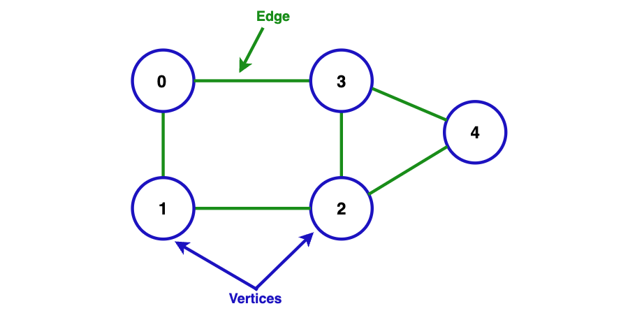
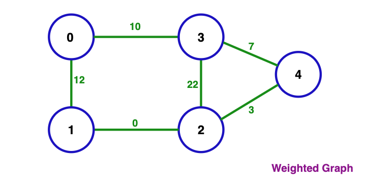
Each edge can also have a value associated with it, called a weight. If all edges
have some weight associated with them, then the graph is called a weighted graph.
There are many different kinds of graphs, and this article won’t cover them all. However there are some important ones that you should know about and you’ll encounter them a lot. It’s important to know the types of graphs because each algorithm works differently on different types of graphs, and some algorithms only work on specific types of graphs.
Let’s look at some common types of graphs:
- Undirected Graph: If the edges between the nodes have no direction, then the graph is called an undirected graph.
- Directed Graph: If the edges between the nodes have a direction, then the graph is called a directed graph.
- Weighted Graph: If the edges between the nodes have some weight associated with them, then the graph is called a weighted graph.
- Cyclic Graph: If there is a cycle in the graph, then the graph is called a cyclic graph. The examples above are cyclic graphs.
- Acyclic Graph: If there is no cycle in the graph, then the graph is called an acyclic graph.
And that’s all there is to it for the basics of graphs! Now let’s move on to how we can represent graphs in code and how we can perform operations on them, most importantly, how we can traverse them.
Graph Representation
There are two main ways to represent a graph in code:
- Adjacency Matrix: An adjacency matrix is a 2D array where the rows represent source nodes and columns represent destination nodes. For unweighted graphs, the matrix will contain 0s and 1s or true and false to represent the connections between the nodes. For weighted graphs, each cell will have a value representing the weight of the edge between two nodes. Let’s see an example:
The adjacency matrix for the unweighted graph in the first figure above. We always set 0 or false for the cells representing the same node.
| 0 | 1 | 2 | 3 | 4 | |
|---|---|---|---|---|---|
| 0 | false | true | false | true | false |
| 1 | true | false | true | false | false |
| 2 | false | true | false | true | true |
| 3 | true | false | true | false | true |
| 4 | false | false | true | true | false |
Now we’re going to try to implement that matrix in Python code:
# Represents unweighted graph - the first image above
adjMatrix = [
    [False, True, False, True, False],
    [True, False, True, False, False],
    [False, True, False, True, True],
    [True, False, True, False, True],
    [False, False, True, True, False]
]

# or we can use 1s and 0s
adjMatrix = [
    [0, 1, 0, 1, 0],
    [1, 0, 1, 0, 0],
    [0, 1, 0, 1, 1],
    [1, 0, 1, 0, 1],
    [0, 0, 1, 1, 0]
]

# both are the same
Now let’s see the adjacency matrix for the weighted graph in the second figure above. We set 0 for the cells representing the same node and we set the weight of the edge between two node for the other cells. But note that a weight value can also be 0 between two different nodes.
So basically a 0 value can represent:
- No edge between two nodes
- An edge between two nodes with a weight of 0
- The same node
Of course, it is not a hard rule, you can use any value you want to represent these as long as you construct your code accordingly. But these are the most common ways to represent these cases.
| 0 | 1 | 2 | 3 | 4 | |
|---|---|---|---|---|---|
| 0 | 0 | 12 | 0 | 10 | 0 |
| 1 | 0 | 0 | 0 | 0 | 0 |
| 2 | 0 | 0 | 0 | 22 | 3 |
| 3 | 0 | 0 | 0 | 0 | 7 |
| 4 | 0 | 0 | 0 | 0 | 0 |
The Python representation of the weighted graph above:
# Represents weighted graph - the second image above
adjMatrix = [
    [0, 12, 0, 10, 0],
    [0, 0, 0, 0, 0],
    [0, 0, 0, 22, 3],
    [0, 0, 0, 0, 7],
    [0, 0, 0, 0, 0]
]
Now that we have seen how to represent a graph using an adjacency matrix, let’s move on to the second way to represent a graph - the adjacency list.
- Adjacency List: An adjacency list is generally a hash map where each key represents a node and the value of the key is a list of all the nodes that are connected to that node. For weighted graphs, the value of the key will be a list of tuples where each tuple contains the node and the weight of the edge between the two nodes. Let’s see how we would represent the unweighted graph from the first figure above using an adjacency list:
| Node | connects with | |||
|---|---|---|---|---|
| 0 | connects with | 1 | 3 | |
| 1 | connects with | 0 | 2 | |
| 2 | connects with | 1 | 3 | 4 |
| 3 | connects with | 0 | 2 | 4 |
| 4 | connects with | 2 | 3 |
The Python representation of the unweighted graph above:
# Represents unweighted graph - the first image above
adjList = {
    0: [1, 3],
    1: [0, 2],
    2: [1, 3, 4],
    3: [0, 2, 4],
    4: [2, 3]
}
Now let’s see the adjacency list for the weighted graph in the second figure above.
| Node | connects with | |||
|---|---|---|---|---|
| 0 | connects with | 1: 12 | 3: 10 | |
| 1 | connects with | 0: 12 | 2: 0 | |
| 2 | connects with | 1: 0 | 3: 22 | 4: 3 |
| 3 | connects with | 0: 10 | 2: 22 | 4: 7 |
| 4 | connects with | 2: 3 | 3: 7 |
The Python representation of the weighted graph above:
# Represents weighted graph - the second image above
adjList = {
    0: [(1, 12), (3, 10)],
    1: [(0, 12), (2, 0)],
    2: [(1, 0), (3, 22), (4, 3)],
    3: [(0, 10), (2, 22), (4, 7)],
    4: [(2, 3), (3, 7)]
}
Great, we’re done with representing two version of a graph. Now next we will look
into some common operations that we can perform on a graph. We will choose the
adjacency list representation for the rest of the article as it is more efficient
and easier to work with. First we will look at how we could construct a graph
in a practical way. It is easy to construct an adjacency list representation
of a graph when we have the graph in front of us. But in reality, we will have
to construct the graph step by step, thus we need a way to do that. For that
we will define a class called WeightedGraph and we will define some methods to add
nodes and edges to the graph. I chose to represent the graph as a weighted graph
because if you understand how to represent a weighted graph, you can easily
understand how to represent an unweighted graph. But I noticed vice versa is not
the case, people struggle to understand how to represent a weighted graph if they
only know how to represent an unweighted graph. Anyway, enough talking, let’s
get to the code.
We will try to create the graph reprsented in the following adjacency list:
adjList = {
    0: [(1, 12), (3, 10)],
    1: [(0, 12), (2, 0)],
    2: [(1, 0), (3, 22), (4, 3)],
    3: [(0, 10), (2, 22), (4, 7)],
    4: [(2, 3), (3, 7)]
}
We first initialize an empty dictionary to store the graph. Then we define a method
add_edge to add a weighted edge to the graph.
class WeightedGraph:
    def __init__(self):
        self.graph = {}

    def add_edge(self, from_node, to_node_tpl):
        if from_node not in self.graph:
            self.graph[from_node] = {}

        self.graph[from_node].append(to_node_tpl)
Here in the code, from_node is just an integer representing the node and to_node_tpl is a tuple where the first value is the node value and the second one is the weight of the edge between the two nodes. We first check if the from_node is already in the graph, if not we add it to the graph. Then we append the to_node to the from_node.
w = WeightedGraph()
w.add_edge(0, (1, 12))
w.add_edge(0, (3, 10))
w.add_edge(1, (0, 12))
w.add_edge(1, (2, 0))
w.add_edge(2, (1, 0))
w.add_edge(2, (3, 22))
w.add_edge(2, (4, 3))
w.add_edge(3, (0, 10))
w.add_edge(3, (2, 22))
w.add_edge(3, (4, 7))
w.add_edge(4, (2, 3))
w.add_edge(4, (3, 7))

print(w.graph)

# Output:
# {0: [(1, 12), (3, 10)], 1: [(0, 12), (2, 0)], 2: [(1, 0), (3, 22), (4, 3)],
# 3: [(0, 10), (2, 22), (4, 7)], 4: [(2, 3), (3, 7)]}
Notice we have to define the edges in both directions. For example to define the edge between 0 and 1, we have to define the edge from 0 to 1 and from 1 to 0.
w.add_edge(0, (1, 12))
w.add_edge(1, (0, 12))
If we only define the edge from 0 to 1, then we cannot traverse from 1 to 0. Our graph is undirected, meaning it is bidirectional.
OK, great! We have successfully created the graph. Now that we have the graph, we can now perform the famous Depth First Search (DFS) and Breadth First Search (BFS) traersal algorithms on the graph.
Graph Traversal
In this section we will look at two different traversal algorithms. To implement the algorithms, we will use two different data structures: a stack for DFS and a queue for BFS. So it is better to quickly check these data structures before we move on to the algorithms.
Depth First Search (DFS)
In DFS, we start from a node and then visit all the nodes connected to that node before moving on to the next node. We keep track of the nodes we have visited at each step, if we already visited the node we skip it.
Let’s see it in example:
class WeightedGraph:
    def __init__(self):
        self.graph = {}

    def add_edge(self, from_node, to_node_tpl):
        if from_node not in self.graph:
            self.graph[from_node] = {}

        self.graph[from_node].append(to_node_tpl)

    def dfs(self, startNode):
        visited = set()

        self.dfs_recursive(startNode, visited)

    def dfs_recursive(self, node, visited):
        if node in visited:
            return

        visited.add(node)

        for child in self.graph[node]:
            to, weight = child
            print(f"Path from {node} to {to} with a weigth {weight}")

            self.dfs_recursive(to, visited)
Here we have defined two methods: dfs and dfs_recursive. The second method
dfs_recursive is a helper method for the first method dfs because we need
to keep track of a state (visited nodes) between the recursive calls and we
don’t want users to pass that state every time they call the method. This way
public method dfs provides cleaner interface by hiding implementation
details. Users only need to provide the starting node, not worrying about the
visited nodes.
So the algorithm is actually really simple, we start from the startNode and
call the dfs_recursive method. In the dfs_recursive method, we first check
if the passed node is visited or not, if it is, we return - the base case. If
not, we add it to the visited nodes set and print the paths from the current
node to the connected nodes. We only print here, but of course you can do
whatever you want with the nodes. You could pass a function to the
dfs_recursive method and call that function with the current node and the
connected nodes, etc. It is up to you. After that, we call the dfs_recursive
method for each connected node. This way we traverse the graph and it is
guaranteed that we visit all the nodes because the graph we are working is
actually a connected graph. If the graph is not connected, then we need to
modify our DFS to ensure we visit all components by iterating through all nodes
in the graph, but we still need to respect the visited set. We would still only
call dfs_recursive on nodes that haven’t been visited yet.
The time complexity of the DFS algorithm is O(V + E) where V is the number of nodes and E is the number of edges in the graph, as we visited each node once and explore each edge once.
So the DFS implementation we’ve seen above is a recursive implementation. As we stated earlier that we could also use a stack to implement the DFS algorithm. Let’s see how we could implement the DFS algorithm using a stack:
class WeightedGraph:
    # ...

    def dfs_stack(self, startNode):
        visited = set()
        stack = [startNode]

        while len(stack) > 0:
            current = stack.pop()

            if current in visited:
                continue

            visited.add(current)

            for child in self.graph[current]:
                to, weight = child
                print(f"Path from {current} to {to} with a weigth {weight}")
                if to not in visited:
                    stack.append(to)
Here we have defined a new method dfs_stack which is the iterative version of
the DFS algorithm. We have a stack where we push the nodes we want to visit. We
start with the startNode and add it to the stack. This is how we initialize
the stack and start popping it - this also gives us the base while condition.
This serves two purposes: First, it gives us our starting point for traversal
and second, it ensures that our while loop condition len(stack) > 0 is
initially true so we can begin processing.
The algorithm then follows a simple pattern.
- Pop the top node from the stack.
- If the node is already visited, skip it.
- If the node is not visited, add it to the visited set.
- Print the path from the current node to the connected nodes.
- Add the connected nodes to the stack if they are not visited yet.
And that’s about it. The time complexity of the iterative version of the DFS algorithm is also O(V + E) where V is the number of nodes and E is the number of edges in the graph.
Now that we have seen the DFS algorithm, let’s move on to the Breadth First
Breadth First Search (BFS)
BFS on the other hand, starts from a node and visits all the nodes connected to that node before moving on to the next level of nodes. Recall that in DFS we go as deep as possible through each path before backtracking. This is the key difference between the two algorithms.
- BFS explores nodes level by level
- DFS explores nodes by following each path to its end before trying other pats
To implement BFS, we will use a queue data structure.
class WeightedGraph:
    # ...

    def bfs(self, startNode):
        visited = set()
        queue = [startNode]

        while len(queue) > 0:
            current = queue.pop(0)

            if current in visited:
                continue

            visited.add(current)

            for child in self.graph[current]:
                to, weight = child
                print(f"Path from {current} to {to} with a weigth {weight}")

                if to not in visited:
                    queue.append(to)
What we did here is very similar to the DFS algorithm in structure, but with
a crucial difference in how we store and process nodes. We have a queue where
we add all the connected nodes to the current node. We start with the
startNode. Since we pop from the queue at the beginning of the loop, after
adding each connected node, at the next step of the loop, we will start to
process the connected nodes. Only difference is that we use a queue instead of
a stack. So basically,
- When we
pop(0)(dequeue) from the queue, we get the earliest added node - When we add all the connected nodes of the current node to the queue, they’ll wait their turn
- Since we added the connected nodes to the end of the queue and we pop from the beginning, we process the nodes in the order they were added, meaning we process all the connected nodes before moving onto the nodes that are one step away from the current node.
Let’s go through a simple example to illustrate this better:
Imagine this graph:
A -> B, C
B -> D, E
C -> F
When we start BGS from A:
- First we put A in the queue:
queue = [A] - We process A and add its children (or connected nodes) B and C to the queue:
queue = [B, C] - Next we process B and add its children D and E to the queue:
queue = [C, D, E] - Finally we process C and add its child F to the queue:
queue = [D, E, F]
and each added nodes are processed in the order they were added. This way we process the nodes in this order: A -> B -> C -> D -> E -> F
The queue basically helps us to keep track of what to visit next.
The time complexity of the BFS algorithm is also O(V + E) where V is the number of nodes and E is the number of edges in the graph.
Summary
In this article we have looked at what a graph is, how we can represent a graph in code, and how we can perform some common operations on a graph. We have looked at two traversal algorithms: Depth First Search (DFS) and Breadth First Search (BFS). We have seen how we can implement these algorithms using both recursive and iterative approaches. We have also seen how we can represent a graph using an adjacency list and how we can construct a graph step by step.